Spreadsheet Tutorial I

Revision 2

Welcome to the spreadsheet tutorial.  Some of you may already own the “Handbook for Sound Engineers: The New Audio Cyclopedia” edited by Glen Ballou.  If you do, please note that the spreadsheet is an improved interactive version of Figure 24-12 in the First Edition, Figure 27-12 in the Second Edition, and Figure 28-25 in the Third Edition.  The descriptions in the text still apply, but many more aspects of the process are contained in the new model.

This spreadsheet displays most of the important factors that govern the performance of an audio tape recorder.  The charts contain plots for each of the individual phenomena and composite curves showing the combined resultant.

Three significant factors that are not yet active are a) eddy current losses, b) resonant peaking, and c) head bumps.  I am still working on those items.

Select the Tabs by clicking on the tabs at the lower left of the screen.

Data

Let’s start out with a tour of the Data tab, the home of all the calculations.  Since these calculations involve logarithms and complex numbers, you will need to install the Excel Analysis Pack that comes with Excel.  You can test your software by typing =COMPLEX(1,1,”j”) in an open cell.  (Copy and Paste didn’t work for me.  Type the entry.)  The result should show 1+j.

In the upper left corner of Data we find all the parameters of the tape recorder.   Many of these variables are named constants, which means they can be called out by name in the formulas rather than RowColumn designations.  The first 6 parameters define the key elements of the recording system.  The starting values are for a recorder operating at 15 ips with NAB equalization – 3180 Hz (50 usec) high end and 50 Hz (3180 usec) low end.

The head gap is set to 200 uin.  Researchers have found that the ‘effective’ gap length of a head is typically 10% to 15% longer than the measured gap.  Several factors may contribute to this ‘stretching’, including rounding of the corners of the pole tips, saturation of the pole tips, and degradation of the magnetic properties of the surface layer of the pole tips in the gap due to the polishing processes used during head construction.  Taking this into account, we are modeling a 180 uin gap, which I believe is the nominal value for the AG-440.  Most professional machines of the middle era used repro gaps of this length as a good compromise for professional tape speeds.  (The later ATR-100 used a 100 uin gap.)

The tape coating thickness, one of the most important parameters in this data, is .55 mils.  Typical studio tapes vary from .5 mils to as much as .68 mils for Scotch 250.  I do not have any data for the European tapes.  Some low print tapes dip down to .4 mils, but more on that later.

The head-to-tape spacing or gap is the effective distance between the head and the tape.  This includes:

1. A work-hardening layer on the face of the head similar to that mentioned in the gap length paragraph above,
2. Any air (and dirt) trapped between the tape and head (a function of tape speed), and
3. The effective roughness of the surface of the tape.

Our newer highly calendared tapes have a highly polished surface that acts as a fairly good mirror!  This has reduced the spacing loss to very low values.  The value of 10 uin used here is from references, not my own experimental data.

The variables for resonant peak frequency and Q of the resonance are currently just ‘place holders’ for future work.

The resistors and capacitors are the components in the AG-440 record circuits for low frequency boost in column D and midband shelving in column E.  Check the value of the boost capacitor.  The circuit uses a .68 uF capacitor.  I accidentally distributed some spreadsheets with a value of .47 uF, a value that more nearly matches the NAB curve.  These values are tied to formulae that model the specific connections of the AG-440.  I also have a similar spreadsheet that has the circuitry for the 3M models 23/56/64.

The plot interval and start frequency determine the frequency array in Column A.  The frequency intervals are twelfth octave.  The end frequency doesn’t do anything yet since I don’t know enough about Excel to have it automatically cover a range.  (Can anyone help me with this?)  I extended the frequencies well beyond the audio range so that the sheet could be used with high-speed machines such as tape duplicators.  If we can incorporate some automatic ranging, we could cut down on the data to just the area of interest.

Gap and Gap dB

We will start with the basics that are displayed in the Gap graph.  This graph will dispel the myth that reproduce gap length is a major factor in determining response.  In fact, at 15 ips and 30 ips, the gap length is rather insignificant.  The only time that it is significant is for Sel Syncing on older machines with broad record heads.

The gap is an aperature – the head’s window to the world.  The magnetic flux linked into the core to produce an output voltage is exactly the flux that is between the boundaries of the gap. 

Imagine that you are the ‘brains’ of the head and that you live in the center of the head core.  Your room has only one window, and it is precisely the area of the gap.  Unfortunately when the low-bid contractor built your room, he used frosted glass from a leftover bathroom window.  When you look out, all you can detect is the average value of the light outside your window.  If someone were to cover half of your window with black cardboard, you would only detect that the total light has dropped to half the unobstructed value.

Passing by your window is a long piece of tape that has vertical stripes of black and white.  If the section in front of your window is totally white, you perceive maximum light; if the section is totally black, totally dark.  If the section has partially white and partially black, you will only perceive the net ‘gray’ value represented by the average over the total window area.  If the patterns are very long compared to the width of the window, you will accurately detect the white or black level of the pattern.  If, however, the vertical bars in the pattern are only half a window wide, you will always detect a constant level of ‘1/2 gray’.

If we assign a number value of 1 to the white area and –1 to the black area, half and half will give an average of zero.

If we continue to make the bars narrower than half the window, we will again have a non-zero average value.  For example, at 1/3 the window width, we might have two white bars and one black bar.  One white bar cancels the black bar, leaving one white bar of 1/3 the window width.  The average is +1/3.  Reversing the colors yields –1/3.  In this case we would see a swing from +1/3 to –1/3 as the tape moves by.

For two pair of bars we would again get ‘1/2 gray’or net zero; three and two bars will give +/-1/5, and so on.

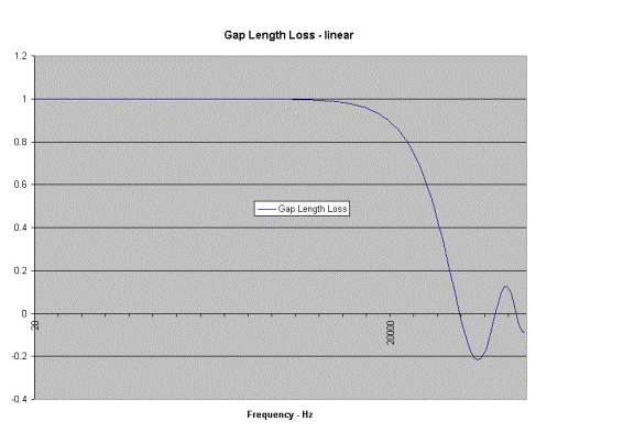
This undulating response can be modeled by the mathematical expression (sine X)/X.  The graph Gap illustrates this phenomenon with a linear vertical scale and log horizontal axis.  The first crossing of the horizontal axis occurs when the wavelength of the signal is exactly equal to the length of the gap (width of our window.)  The second crossing is at two wavelengths equal the gap length, and so on.  Note that the polarity changes back and forth, with positive peaks at 5, 9, 13,… half cycles or bars,  and negative peaks at 3, 7, 11,… half cycles.

If we replot this curve using a logarithmic vertical axis, we get the graph Gap dB.  Here we see the zero crossings as chasms that drop to minus infinity on the dB scale.  We can’t take the logarithm of a negative number, so we had to throw away the polarity information before taking the log.

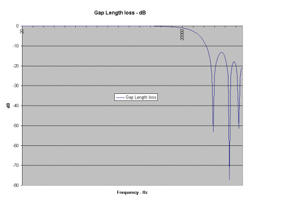
We can look at the gap length losses by placing the cursor on a data point of the curve.  For example, scan along the curve until you find Point 121 with a value of –1.04 dB.  We can convert this to an exact frequency using the Data sheet.  The data starts at line 20, so we must add 19 to the number of the point, in this case 19 + 121 = 140.  If we look at line 140 in the Sheet 1 we find a frequency of 20 k Hz in Column A and a gap length loss of –1.04 dB in Column H.

This tells us that for our AG-440 at 15 ips, we have at most 1 dB of loss due to the gap length in the audio band from 20 Hz to 20 kHz!  That is really quite insignificant!

You might want to take this opportunity to change the value for tape speed in the spreadsheet and check the results.  At 30 ips the maximum loss drops to about .25 dB, but at 7.5 ips it shoots up to 4.5 dB.  Whoa!  That is no longer insignificant!  Trying to get 20 kHz out of a 200 uin head is not a good idea if you want flat response.  A 100 uin gap, on the other hand, would give us the 1 dB loss at 7.5 ips that we saw with the 200 uin gap at 15 ips.

Why not use the narrowest gap possible for all tape speeds?  Expense is only a minor consideration.  More importantly, as we make the gap shorter, we increase the amount of flux that never gets to the sensing coils.  A portion of the flux prefers to take a ‘shortcut’ and just loops into the gap without traversing the long path through the core and coils.  The narrower the gap is, the more flux we have shortcutting.  This reduction in signal compromises our signal-to-noise ratio.

We are left with the compromise of long gaps for maximum signal-to-noise ratio, short gaps for high frequencies at slow speeds.  (Instrumentation machines running at 240 ips may use gaps of 30 uin to achieve frequency response out to 2 MHz.  You can try that combination in the model.)

Head & Tape

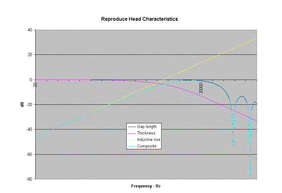
If you were to hook up a reproduce head directly to a voltmeter and run a tape with a frequency sweep across the head, you would generate the graph Head & Tape.  The yellow curve is a simple 6 dB per octave rise due to the inductive nature of the head.  The output voltage from the head depends upon the magnetic structure, the number of turns on the head coils, and the rate of change of flux at the gap.  Higher frequencies change flux faster, so the voltage goes up with frequency.  Without any eddy current losses, this is a straight line.

We can generate this curve on our tape recorder by using a flux loop.  The flux loop is simply a coil in front of the gap that turns the head into a transformer rather than a wavelength-dependent transducer.  If we drive the loop with a sinewave oscillator, holding the current in the coil of the loop constant as we sweep frequency, the flux from the loop will be constant.  The resulting head voltage will rise at the 6 dB per octave rate less any eddy current losses.

The violet curve is the thickness loss curve.  Unfortunately, the reproduce head is ‘nearsighted’.  It can see the tightly packed flux reversals very clearly at the surface of the head, but things blur out as the head tries to look deeper into the oxide layer.  The tighter        we make the packing (due to increased frequency), the greater the loss due to this nearsightedness.  THIS IS THE MOST IMPORTANT LOSS FOR AN AUDIO MACHINE!

We can look at the losses by placing the cursor on a data point of the curve.  For example, scan along the curve until you find Point 70 with a value of –1.04 dB.  We can convert this to an exact frequency using Data.  The frequency incrementing starts at line 20, so we must add 19 to the number of the point, in this case 19 + 70 = 89.  If we look at line 89 in the Sheet 1 we find a frequency of 1,062 Hz in Column A and a thickness loss of –1.04 dB in Column I.

Gad zooks!  We have already lost 1 dB by the time we are at a kilohertz!   Now our gap length losses really do look trivial!

The low frequency part of the violet curve is the area in which all of the flux is read by the gap.  We use this portion of the curve to set the proper level on the record gain pot.  This output level will vary with the thickness of the tape, either from type to type or from batch to batch. 

Since we most commonly use an alignment tape to set the reproduce gain pot, we are not affected by changes in oxide thickness on the test tape.  Jay McKnight has already taken care of that for us in setting his record level to give us the proper amount of flux for whatever coating thickness is on that specific piece of tape.

Above approximately 1 kHz the thickness loss takes control, canceling out the inductive rise.  The thickness loss continues to dominate until we reach 20 kHz, at which point we have gone past 1 dB on the gap length loss (sine X)/X curve.  The head voltage dives into the abyss of the first gap length null.  The light blue curve shows the composite response for all these factors.

This humped output curve has been the standard data provided by head manufacturers.  Most people don’t realize that much of the shape of this curve is dictated by the coating thickness of the tape used to generate the curve.

The key factor determining the shape of the curve is the ratio of the gap length to the tape coating thickness.  If the thickness is about two and one half times the gap length, as with an AG-440, the response is a hump.  For the ATR-100, however, the ratio is closer to 5 and the graph has a broad plateau that is flat within 2 dB over a decade of frequencies.

Flux

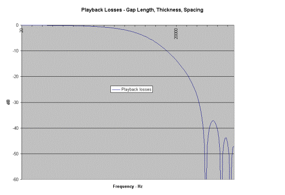
If we remove the inductive rise from our discussion and re-plot the data for thickness and gap length loss, we get the Flux graph.  This shows that we have serious high frequency problems that we must correct.  Our obvious first choice is to put in equalization that rises at high frequencies to compensate for the losses.  Our first choice would be a simple RC circuit.  Ahh, if life were just that simple….

Thickness vs RC

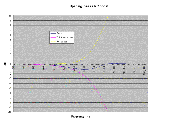
Our model allows us to test the practicality of balancing the thickness loss with an RC circuit.  The Thickness vs RC graph shows us the sum of the thickness loss and an RC boost.  You can try varying the RC boost frequency by changing the value in cell D3   My value of 4340 Hz was chosen to give good correction at low and high frequencies.

Boy, are we screwed!  The shapes of the two curves don’t match!  The transition regions are following different types of mathematical curves.  The thickness loss expression contains exponential terms, but the RC curve has only squares and square roots.  They just don’t match.

In our example we are stuck with a 1.14 dB hole at 2667 Hz, right in the middle of our audio band.  No matter how you juggle the values, you can’t cancel this hole with a simple RC circuit.  Oh sure, you can slide it around to split the difference.  For example, try an RC frequency of 3900 Hz.  This makes the downward loop a little bit less, but inserts a +1 dB error at high frequencies.  Moving up to 5200 Hz pulls everything down so that it looks like a shelf.  Our 3180 Hz NAB standard pushes everything up to create a shelf at +2.7 dB, but we still have a .6 dB hole around 1300 Hz.  Some days you just can’t win!

Leave the value of cell D3 at 3180 Hz for the next section.

Boost & Shelf

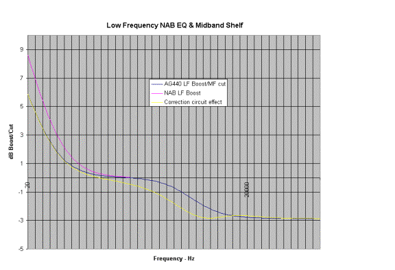
As we have seen, we are in trouble because of the different shapes of the thickness loss and RC boost curves.  In the mid 60’s manufacturers started to put midband shelving circuits into the record amplifiers to try to correct the mismatch.  The Boost & Shelf curves show the frequency response of the AG-440’s attempt to solve this problem.  The blue curve is the response of the circuit, and the yellow curve adds in the mismatch curve from the previous graph.  We still have a dip of 1.3 dB in the midband at 3 kHz.

If we are lucky, we might have some high frequency losses that will pull the top end down a dB or more, allowing us to apply a bit of high frequency record equalization to lift things up.

The AG-440 low frequency boost circuit is also a problem.  The violet curve is the 50 Hz target for the NAB standard.  Try changing the boost capacitor value in cell D14 to .47 uF to reduce the error.

TOTAL

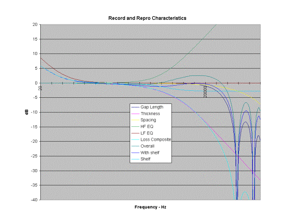
If we add all of these effects together, we get the traces shown on the TOTAL graph.  The blue curve titled ‘with shelf’ is the composite of everything above.  Aside from the midband dip of 1.2 dB, the response is quite good.  The low frequency boost doesn’t match the 50 Hz NAB boost, but we know how to fix that.

What hasn’t been included

We haven’t included any high frequency record equalization in our model!  If the playback equalization truly matches the tape’s coating thickness characteristics, we approach ‘constant current recording.’  The current drive to the record head is constant at all audio frequencies across the audio band (except for the deliberate boost at low frequencies dictated by the NAB standard.)

Our low end response will change drastically due to head bumps.  Separating the head bump response from the inherent low frequency response can be daunting.  A full track test tape certainly confuses things with fringing that is somewhat dependent on the track format, the track location and the construction and shielding of the head.

Eddy currents will cause a droop at high frequencies.  The amount of droop will be different for the 6 mil head laminations of the AG-440’A’ and AG-440B (and MM-1000?) compared to the 2 mil laminations of the AG-440 C and the MM-1100/1200.  The AG-440 head transformer also has eddy current losses.  Eddy currents affect both record and play functions. 

Resonances will also change the response at both high and low frequencies.  At high frequencies the head inductance (and transformer inductance if a head transformer is used) combines with the head, cable, input stage (and transformer) capacitances to create a resonance near the top of the audio band.  On some machines this resonant rise is use to offset gap length and other losses.

At low frequencies the output transformer may series resonate with the output amplifier coupling capacitor.  Once again, this resonance may be used to flatten the overall response.

The input and output transformers may also have ringing at high frequencies.

In general, using resonant circuits to flatten the response will compromise the transient response of the system.  Circuits without such resonances are generally judged as ‘tighter’ and less strident.  If a resonance is unavoidable, then careful damping of the resonance can minimize its effect.  Transient testing with squarewaves and bursts is usually required for this optimization.